Predicting pileups: Using ML to predict Chicago crash types
By Jeremy R. Winget in Blog
December 18, 2021
Wouldn’t it be great to know the chances of being injured or having your car totaled in a car accident before ever being involved in the accident? If you live in a less densely populated area, this question might not be very interesting. But if you live in a big city, like Chicago, you might be a little more concerned about this. By identifying factors that predict these bad accidents, we might be able to develop low cost interventions or redesign the environment to reduce the frequency of these types of accidents, which can translate to lives and money saved. So in this post, we’ll use machine learning to predict which traffic crashes in Chicago, IL, result in injuries and/or the vehicle being towed based on situational features (e.g., posted speed limit, lighting conditions, road surface condition, etc.) that are likely known before the crash occurred.
Traffic crash data were imported from the Chicago Data Portal using the RSocrata package. The City of Chicago also has data sets related to the vehicles and people involved in these crashes, but to keep things simple for now, let’s focus on a few situational factors related to the crash, all of which can be found in the main data set.
These data show information about each traffic crash on city streets within the City of Chicago and under the jurisdiction of the Chicago Police Department. Many of the variables (e.g. street conditions, weather conditions, etc.) are recorded by the reporting officer and are based on the best available information at the time, but according to the Chicago Data Portal, these data may disagree with other posted information. As such, data are subject to change based on new information.
Import data
set.seed(20211218)
library(RSocrata)
library(tidyverse)
library(lubridate)
library(janitor)
library(tidymodels)
library(vip)
library(skimr, include.only = "skim")

# data pulled at time of post; new cases likely added to data portal since then
crashes <- read.socrata(
  "https://data.cityofchicago.org/resource/85ca-t3if.csv", # url of data set
  app_token = Sys.getenv("rsocrata_token")                 # my personal creds
) %>%
  clean_names() %>%
  select(
    crash_type, crash_date, posted_speed_limit, traffic_control_device,
    device_condition, weather_condition, lighting_condition, first_crash_type,
    trafficway_type, alignment, roadway_surface_cond, road_defect, prim_contributory_cause
  ) %>%
  mutate(
    crash_date = ymd_hms(crash_date),
    date = as_date(crash_date)
  ) %>%
  select(!crash_date)
The goal here is to build a model that predicts whether a crash will result in someone being injured and/or the vehicle being towed using the crash_type variable in the crashes data set.
From the variables listed in the
Traffic Crash data set, let’s select some that are likely to have been known before the crash occurred. For example, lighting_condition is a variable that records the light condition at the time of the crash. This situational factor is likely to be known (e.g., observed by the driver, reported by others prior to the crash, etc.) before an accident occurs. At the very least, this information has a higher chance of being known prior to a crash compared to something like injuries_total. injuries_total is a variable that records the total number of people who sustained an injury as a result of the accident. Since this is a consequence of a crash, this information can only known after the crash occurs.
With this logic, let’s focus on the following variables from the initial Traffic Crash data set:
| Column name | Description | Type |
|---|---|---|
| crash_date | Date and time of crash as entered by the reporting officer | Date/Time |
| posted_speed_limit | Posted speed limit, as determined by reporting officer | Numeric |
| traffic_control_device | Traffic control device present at crash location, as determined by reporting officer | Factor |
| device_condition | Condition of traffic control device, as determined by reporting officer | Factor |
| weather_condition | Weather condition at time of crash, as determined by reporting officer | Factor |
| lighting_condition | Light condition at time of crash, as determined by reporting officer | Factor |
| first_crash_type | Type of first collision in crash | Factor |
| trafficway_type | Trafficway type, as determined by reporting officer | Factor |
| alignment | Street alignment at crash location, as determined by reporting officer | Factor |
| roadway_surface_cond | Road surface condition, as determined by reporting officer | Factor |
| road_defect | Road defects, as determined by reporting officer | Factor |
| prim_contributory_cause | The factor which was most significant in causing the crash, as determined by officer judgment | Factor |
Data exploration & cleaning
Now that we have some idea of what we’ll be looking at in our model, let’s get some impressions of the data and see if anything needs to be cleaned up before going further.
glimpse(crashes)
Rows: 571,184
Columns: 13
$ crash_type              <chr> "NO INJURY / DRIVE AWAY", "INJURY AND / OR TOW…
$ posted_speed_limit      <int> 30, 30, 30, 30, 35, 30, 30, 30, 20, 20, 30, 30…
$ traffic_control_device  <chr> "NO CONTROLS", "STOP SIGN/FLASHER", "TRAFFIC S…
$ device_condition        <chr> "NO CONTROLS", "FUNCTIONING PROPERLY", "FUNCTI…
$ weather_condition       <chr> "CLEAR", "CLEAR", "CLEAR", "CLEAR", "CLEAR", "…
$ lighting_condition      <chr> "DARKNESS, LIGHTED ROAD", "DAYLIGHT", "DAYLIGH…
$ first_crash_type        <chr> "REAR END", "ANGLE", "TURNING", "ANGLE", "TURN…
$ trafficway_type         <chr> "ONE-WAY", "DIVIDED - W/MEDIAN (NOT RAISED)", …
$ alignment               <chr> "STRAIGHT AND LEVEL", "STRAIGHT AND LEVEL", "S…
$ roadway_surface_cond    <chr> "DRY", "DRY", "DRY", "DRY", "DRY", "DRY", "UNK…
$ road_defect             <chr> "NO DEFECTS", "UNKNOWN", "NO DEFECTS", "NO DEF…
$ prim_contributory_cause <chr> "IMPROPER OVERTAKING/PASSING", "FAILING TO RED…
$ date                    <date> 2019-08-21, 2016-09-20, 2018-04-16, 2018-04-2…
The first thing to note is that there are 571426 observations with 13 columns in the crashes data set. And other than some potential capitalization issues with the strings, there doesn’t seem to be any obvious issues with the way the data are formatted. We’ll come back to this, but for now, let’s check for missing data.
colSums(is.na(crashes))
             crash_type      posted_speed_limit  traffic_control_device
                      0                       0                       0
       device_condition       weather_condition      lighting_condition
                      0                       0                       0
       first_crash_type         trafficway_type               alignment
                      0                       0                       0
   roadway_surface_cond             road_defect prim_contributory_cause
                      0                       0                       0
                   date
                      0
Great, no missing data! This will simplify data preparation later on. Next, we should examine the frequency counts of the variables we’ll use to predict the outcome class.
var_freq <- function(df) {
  map(names(df), ~ count(df, .data[[.x]]))[1:12]
}

var_freq(crashes)
[[1]]
                        crash_type      n
1 INJURY AND / OR TOW DUE TO CRASH 146704
2           NO INJURY / DRIVE AWAY 424722

[[2]]
   posted_speed_limit      n
1                   0   6967
2                   1     37
3                   2     22
4                   3    135
5                   4      2
6                   5   3982
7                   6      7
8                   7      2
9                   9     94
10                 10  12618
11                 11      8
12                 12      3
13                 14      3
14                 15  20184
15                 16      1
16                 18      2
17                 20  23046
18                 22      2
19                 23      1
20                 24     29
21                 25  35213
22                 26      2
23                 29      1
24                 30 420252
25                 31      2
26                 32     15
27                 33     11
28                 34     13
29                 35  39110
30                 36      5
31                 38      2
32                 39     62
33                 40   5287
34                 45   3513
35                 49      1
36                 50    133
37                 55    545
38                 60     32
39                 63      1
40                 65     12
41                 70      3
42                 99     66

[[3]]
     traffic_control_device      n
1     BICYCLE CROSSING SIGN     17
2               DELINEATORS    191
3   FLASHING CONTROL SIGNAL    182
4          LANE USE MARKING   1226
5               NO CONTROLS 328889
6                NO PASSING     26
7                     OTHER   3505
8   OTHER RAILROAD CROSSING    137
9           OTHER REG. SIGN    591
10       OTHER WARNING SIGN    513
11 PEDESTRIAN CROSSING SIGN    275
12           POLICE/FLAGMAN    206
13   RAILROAD CROSSING GATE    374
14         RR CROSSING SIGN     66
15              SCHOOL ZONE    188
16        STOP SIGN/FLASHER  56828
17           TRAFFIC SIGNAL 158633
18                  UNKNOWN  18773
19                    YIELD    806

[[4]]
          device_condition      n
1   FUNCTIONING IMPROPERLY   2913
2     FUNCTIONING PROPERLY 197610
3                  MISSING     68
4              NO CONTROLS 332457
5          NOT FUNCTIONING   1854
6                    OTHER   4442
7                  UNKNOWN  31851
8 WORN REFLECTIVE MATERIAL    231

[[5]]
          weather_condition      n
1  BLOWING SAND, SOIL, DIRT      2
2              BLOWING SNOW    169
3                     CLEAR 454044
4           CLOUDY/OVERCAST  16937
5            FOG/SMOKE/HAZE    858
6     FREEZING RAIN/DRIZZLE    701
7                     OTHER   1732
8                      RAIN  50003
9    SEVERE CROSS WIND GATE    116
10               SLEET/HAIL    736
11                     SNOW  20386
12                  UNKNOWN  25742

[[6]]
      lighting_condition      n
1               DARKNESS  28092
2 DARKNESS, LIGHTED ROAD 124367
3                   DAWN   9773
4               DAYLIGHT 370366
5                   DUSK  17184
6                UNKNOWN  21644

[[7]]
               first_crash_type      n
1                         ANGLE  61096
2                        ANIMAL    400
3                  FIXED OBJECT  26634
4                       HEAD ON   4918
5            OTHER NONCOLLISION   1828
6                  OTHER OBJECT   5501
7                    OVERTURNED    345
8          PARKED MOTOR VEHICLE 132917
9                  PEDALCYCLIST   8437
10                   PEDESTRIAN  13077
11                     REAR END 133128
12                REAR TO FRONT   4027
13                 REAR TO REAR    886
14                 REAR TO SIDE   2413
15 SIDESWIPE OPPOSITE DIRECTION   8319
16     SIDESWIPE SAME DIRECTION  87334
17                        TRAIN     36
18                      TURNING  80130

[[8]]
                   trafficway_type      n
1                            ALLEY   9369
2                 CENTER TURN LANE   4602
3  DIVIDED - W/MEDIAN (NOT RAISED)  98035
4       DIVIDED - W/MEDIAN BARRIER  33689
5                         DRIVEWAY   1953
6              FIVE POINT, OR MORE    574
7                         FOUR WAY  23286
8                   L-INTERSECTION     80
9                      NOT DIVIDED 253000
10                    NOT REPORTED    214
11                         ONE-WAY  75267
12                           OTHER  15948
13                     PARKING LOT  39919
14                            RAMP   1793
15                      ROUNDABOUT    139
16                  T-INTERSECTION   4950
17                   TRAFFIC ROUTE    436
18                         UNKNOWN   6310
19       UNKNOWN INTERSECTION TYPE   1293
20                  Y-INTERSECTION    569

[[9]]
              alignment      n
1        CURVE ON GRADE    853
2    CURVE ON HILLCREST    272
3          CURVE, LEVEL   4335
4    STRAIGHT AND LEVEL 557037
5     STRAIGHT ON GRADE   7225
6 STRAIGHT ON HILLCREST   1704

[[10]]
  roadway_surface_cond      n
1                  DRY 430091
2                  ICE   3943
3                OTHER   1375
4      SAND, MUD, DIRT    241
5        SNOW OR SLUSH  20443
6              UNKNOWN  39264
7                  WET  76069

[[11]]
        road_defect      n
1 DEBRIS ON ROADWAY    478
2        NO DEFECTS 472661
3             OTHER   3214
4        RUT, HOLES   4855
5   SHOULDER DEFECT   1212
6           UNKNOWN  86671
7      WORN SURFACE   2335

[[12]]
                                                            prim_contributory_cause
1                                                                            ANIMAL
2                                            BICYCLE ADVANCING LEGALLY ON RED LIGHT
3                                                 CELL PHONE USE OTHER THAN TEXTING
4                                                  DISREGARDING OTHER TRAFFIC SIGNS
5                                                        DISREGARDING ROAD MARKINGS
6                                                            DISREGARDING STOP SIGN
7                                                      DISREGARDING TRAFFIC SIGNALS
8                                                           DISREGARDING YIELD SIGN
9                                                 DISTRACTION - FROM INSIDE VEHICLE
10                                               DISTRACTION - FROM OUTSIDE VEHICLE
11      DISTRACTION - OTHER ELECTRONIC DEVICE (NAVIGATION DEVICE, DVD PLAYER, ETC.)
12                                                  DRIVING ON WRONG SIDE/WRONG WAY
13                                              DRIVING SKILLS/KNOWLEDGE/EXPERIENCE
14                                                    EQUIPMENT - VEHICLE CONDITION
15                                EVASIVE ACTION DUE TO ANIMAL, OBJECT, NONMOTORIST
16                                                 EXCEEDING AUTHORIZED SPEED LIMIT
17                                              EXCEEDING SAFE SPEED FOR CONDITIONS
18                                           FAILING TO REDUCE SPEED TO AVOID CRASH
19                                                    FAILING TO YIELD RIGHT-OF-WAY
20                                                            FOLLOWING TOO CLOSELY
21                                  HAD BEEN DRINKING (USE WHEN ARREST IS NOT MADE)
22                                                                 IMPROPER BACKING
23                                                              IMPROPER LANE USAGE
24                                                      IMPROPER OVERTAKING/PASSING
25                                                       IMPROPER TURNING/NO SIGNAL
26                                        MOTORCYCLE ADVANCING LEGALLY ON RED LIGHT
27                                                                   NOT APPLICABLE
28                                                            OBSTRUCTED CROSSWALKS
29 OPERATING VEHICLE IN ERRATIC, RECKLESS, CARELESS, NEGLIGENT OR AGGRESSIVE MANNER
30                                                       PASSING STOPPED SCHOOL BUS
31                                                     PHYSICAL CONDITION OF DRIVER
32                                                              RELATED TO BUS STOP
33                                                    ROAD CONSTRUCTION/MAINTENANCE
34                                         ROAD ENGINEERING/SURFACE/MARKING DEFECTS
35                                                                          TEXTING
36                                                             TURNING RIGHT ON RED
37                                                              UNABLE TO DETERMINE
38               UNDER THE INFLUENCE OF ALCOHOL/DRUGS (USE WHEN ARREST IS EFFECTED)
39                             VISION OBSCURED (SIGNS, TREE LIMBS, BUILDINGS, ETC.)
40                                                                          WEATHER
        n
1     486
2      72
3     803
4    1238
5     764
6    6450
7   10785
8     213
9    4132
10   2514
11    277
12   2837
13  18131
14   3658
15   1083
16   1982
17   1684
18  24758
19  62495
20  58791
21    630
22  24242
23  21609
24  27301
25  18880
26     19
27  30637
28     47
29   7318
30     76
31   3467
32    213
33   1348
34   1500
35    250
36    403
37 214923
38   2972
39   3382
40   9056
Looks like there are some issues that need to be addressed here! First, the responses that are coded for some variables don’t make sense. For example, posted_speed_limit has 6967 recorded observations for a posted speed limit of 0 mph. Clearly, this is not a legitimate posted speed limit within the City of Chicago (as much as it may feel like it on the Dan Ryan at 5pm). There are some other odd speed limits recorded for this variable as well.
Another issue these frequency counts reveal is that many of the levels within a variable could be grouped together. For example, prim_contributory_cause makes a distinction between disregarding road markings, stop signs, traffic signals, yield signs, and other traffic signs. Instead, these levels could be grouped into a single level called “disregarding signs/markings”.
So, let’s address each of these problems by cleaning up the levels for each variable. And while we’re at it, let’s clean up the format of all of the strings so there is a consistent style (i.e., lower case).
crashes <- crashes %>%
  mutate(
    across(where(is.character), ~ str_to_lower(.)),
    traffic_control_device = case_when(
      traffic_control_device == "railroad crossing gate" |
       traffic_control_device == "other railroad crossing" |
        traffic_control_device == "rr crossing sign" ~ "rr crossing",
      traffic_control_device == "bicycle crossing sign" |
        traffic_control_device == "pedestrian crossing sign" |
        traffic_control_device == "school zone" ~ "pedestrian signs",
      traffic_control_device == "flashing control signal" ~ "stop sign/flasher",
      traffic_control_device == "no passing" ~ "other warning sign",
      TRUE ~ traffic_control_device
    ),
    device_condition = case_when(
      device_condition == "missing" ~ "no controls",
      device_condition == "worn reflective material" |
        device_condition == "not functioning" ~ "functioning improperly",
      TRUE ~ device_condition
    ),
    weather_condition = case_when(
      weather_condition == "blowing sand, soil, dirt" |
        weather_condition == "severe cross wind gate" |
        weather_condition == "blowing snow" ~ "blowing debris",
      weather_condition == "freezing rain/drizzle" |
        weather_condition == "sleet/hail" ~ "sleet/hail/freezing rain",
      TRUE ~ weather_condition
    ),
    prim_contributory_cause = case_when(
      prim_contributory_cause == "disregarding other traffic signs" |
        prim_contributory_cause == "disregarding road markings" |
        prim_contributory_cause == "disregarding stop sign" |
        prim_contributory_cause == "disregarding traffic signals" |
        prim_contributory_cause == "disregarding yield sign" |
        prim_contributory_cause == "passing stopped school bus" ~ "disregarding signs/markings",
      prim_contributory_cause == "distraction - from inside vehicle" |
        prim_contributory_cause == "distraction - from outside vehicle" |
        prim_contributory_cause == "distraction - other electronic device (navigation device, dvd player, etc.)" |
        prim_contributory_cause == "cell phone use other than texting" |
        prim_contributory_cause == "texting" ~ "distraction",
      prim_contributory_cause == "had been drinking (use when arrest is not made)" |
        prim_contributory_cause == "under the influence of alcohol/drugs (use when arrest is effected)" ~ "under the influence",
      prim_contributory_cause == "obstructed crosswalks" |
        prim_contributory_cause == "vision obscured (signs, tree limbs, buildings, etc.)" ~ "obstructions",
      prim_contributory_cause == "bicycle advancing legally on red light" |
        prim_contributory_cause == "motorcycle advancing legally on red light" ~ "bike/motorcycle advancing legally on red light",
      prim_contributory_cause == "animal" |
        prim_contributory_cause == "evasive action due to animal, object, nonmotorist" ~ "evasive action",
      prim_contributory_cause == "exceeding authorized speed limit" |
        prim_contributory_cause == "exceeding safe speed for conditions" ~ "speeding",
      TRUE ~ prim_contributory_cause
    ),
    across(where(is_character), ~ as_factor(.))
  )
Great! Now, the data are clean, and we can start thinking about how to set up the model. Let’s take a look at the current data summary.
skim(crashes)
Table: Table 1: Data summary
| Name | crashes |
| Number of rows | 571184 |
| Number of columns | 13 |
| _______________________ | |
| Column type frequency: | |
| Date | 1 |
| factor | 11 |
| numeric | 1 |
| ________________________ | |
| Group variables | None |
Variable type: Date
| skim_variable | n_missing | complete_rate | min | max | median | n_unique |
|---|---|---|---|---|---|---|
| date | 0 | 1 | 2013-03-03 | 2021-12-16 | 2019-04-04 | 2360 |
Variable type: factor
| skim_variable | n_missing | complete_rate | ordered | n_unique | top_counts |
|---|---|---|---|---|---|
| crash_type | 0 | 1 | FALSE | 2 | no : 424559, inj: 146625 |
| traffic_control_device | 0 | 1 | FALSE | 13 | no : 328744, tra: 158581, sto: 56983, unk: 18764 |
| device_condition | 0 | 1 | FALSE | 5 | no : 332373, fun: 197537, unk: 31837, fun: 4996 |
| weather_condition | 0 | 1 | FALSE | 9 | cle: 453842, rai: 49987, unk: 25729, sno: 20386 |
| lighting_condition | 0 | 1 | FALSE | 6 | day: 370247, dar: 124277, dar: 28081, unk: 21635 |
| first_crash_type | 0 | 1 | FALSE | 18 | rea: 133081, par: 132866, sid: 87296, tur: 80093 |
| trafficway_type | 0 | 1 | FALSE | 20 | not: 252898, div: 97994, one: 75242, par: 39894 |
| alignment | 0 | 1 | FALSE | 6 | str: 556802, str: 7219, cur: 4334, str: 1704 |
| roadway_surface_cond | 0 | 1 | FALSE | 7 | dry: 429895, wet: 76044, unk: 39245, sno: 20443 |
| road_defect | 0 | 1 | FALSE | 7 | no : 472466, unk: 86626, rut: 4855, oth: 3213 |
| prim_contributory_cause | 0 | 1 | FALSE | 26 | una: 214837, fai: 62463, fol: 58770, not: 30619 |
Variable type: numeric
| skim_variable | n_missing | complete_rate | mean | sd | p0 | p25 | p50 | p75 | p100 | hist |
|---|---|---|---|---|---|---|---|---|---|---|
| posted_speed_limit | 0 | 1 | 28.33 | 6.37 | 0 | 30 | 30 | 30 | 99 | ▁▇▁▁▁ |
And, let’s take a closer look at the dependent variable, crash_type.
crashes %>%
  count(crash_type) %>%
  mutate(prop = n / sum(n))
                        crash_type      n      prop
1           no injury / drive away 424559 0.7432964
2 injury and / or tow due to crash 146625 0.2567036
It looks like there might be a bit of imbalance in the data since the class proportions are skewed towards non-injury/drive-away (74.3%) crash types. Imbalance can sometimes lead to problems in an analysis, especially in severe cases of imbalance. Fortunately, there are a few approaches that try to mitigate this issue (e.g., themis). For now, let’s just analyze the data as is.
At this point, it would be helpful to know which variables in the crashes data set are associated with the different levels of the dependent variable, crash_type. One quick way of doing this for the numeric predictors is by using box plots.
crashes %>%
  ggplot(aes(x = crash_type, y = posted_speed_limit, fill = crash_type)) +
  geom_boxplot()
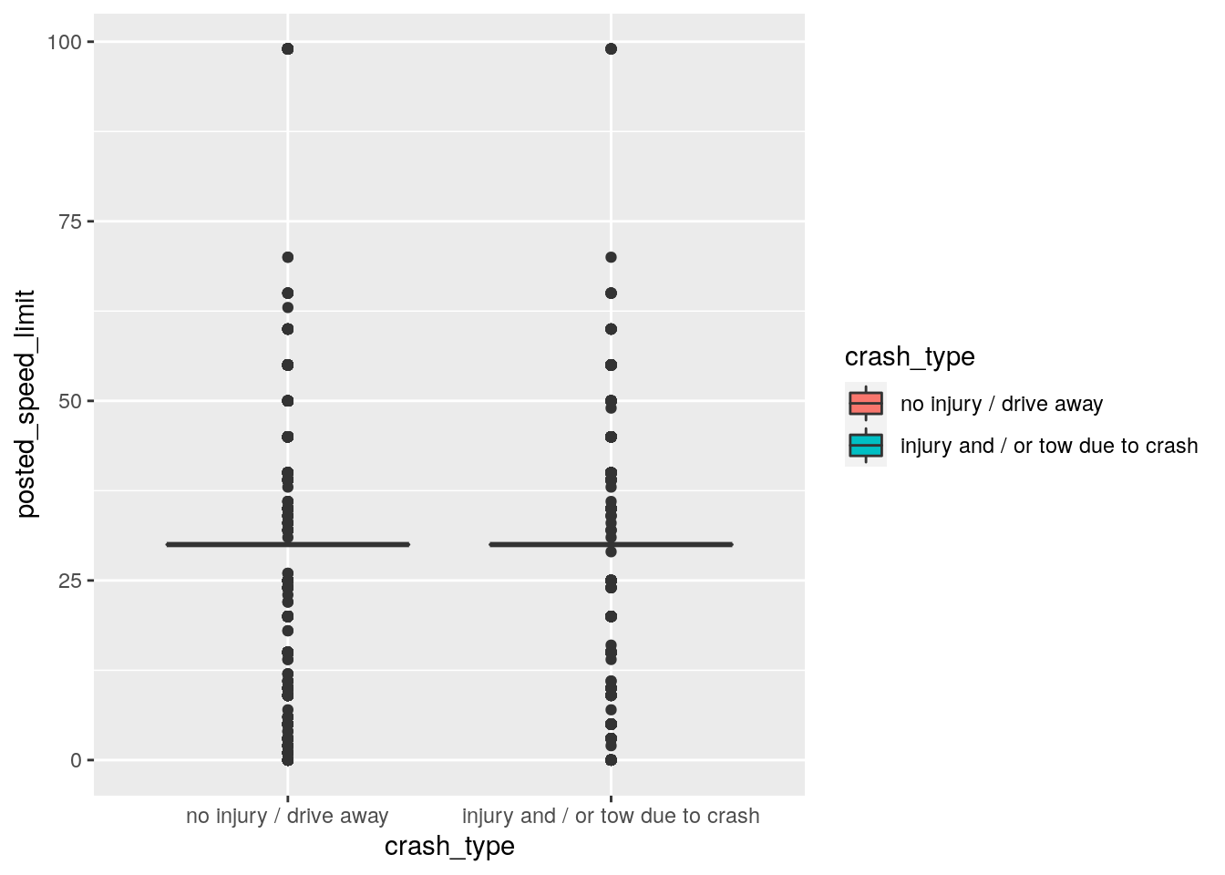
It looks like any differences between the crash_type levels are quite small for posted_speed_limit. So, maybe this variable won’t be so helpful in predicting injuries/towed crash types after all.
Next, let’s check the the relationship between the categorical variables and crash_type using simple counts. We’ll also filter for counts that are at least 1% of the total proportion of observations to get a better idea of the larger data patterns.
print_counts <- function(.y_var) {
  y_var <- sym(.y_var)

  crashes %>%
    count(crash_type, {{y_var}}) %>%
    group_by(crash_type) %>%
    mutate(percent = round_half_up(n / sum(n) * 100, 2))
}

y_var <- crashes %>%
  select(where(is.factor), -crash_type) %>%
  variable.names()

map(y_var, print_counts) %>%
  map(., ~ filter(., percent > 1))
[[1]]
# A tibble: 8 × 4
# Groups:   crash_type [2]
  crash_type                       traffic_control_device      n percent
  <fct>                            <fct>                   <int>   <dbl>
1 no injury / drive away           no controls            256324   60.4
2 no injury / drive away           stop sign/flasher       35711    8.41
3 no injury / drive away           traffic signal         111530   26.3
4 no injury / drive away           unknown                 15550    3.66
5 injury and / or tow due to crash no controls             72420   49.4
6 injury and / or tow due to crash stop sign/flasher       21272   14.5
7 injury and / or tow due to crash traffic signal          47051   32.1
8 injury and / or tow due to crash unknown                  3214    2.19

[[2]]
# A tibble: 7 × 4
# Groups:   crash_type [2]
  crash_type                       device_condition            n percent
  <fct>                            <fct>                   <int>   <dbl>
1 no injury / drive away           no controls            258832   61.0
2 no injury / drive away           functioning properly   134448   31.7
3 no injury / drive away           unknown                 24928    5.87
4 injury and / or tow due to crash no controls             73541   50.2
5 injury and / or tow due to crash functioning properly    63089   43.0
6 injury and / or tow due to crash functioning improperly   1690    1.15
7 injury and / or tow due to crash unknown                  6909    4.71

[[3]]
# A tibble: 10 × 4
# Groups:   crash_type [2]
   crash_type                       weather_condition      n percent
   <fct>                            <fct>              <int>   <dbl>
 1 no injury / drive away           clear             338172   79.6
 2 no injury / drive away           snow               15085    3.55
 3 no injury / drive away           rain               33841    7.97
 4 no injury / drive away           unknown            22999    5.42
 5 no injury / drive away           cloudy/overcast    11782    2.78
 6 injury and / or tow due to crash clear             115670   78.9
 7 injury and / or tow due to crash snow                5301    3.62
 8 injury and / or tow due to crash rain               16146   11.0
 9 injury and / or tow due to crash unknown             2730    1.86
10 injury and / or tow due to crash cloudy/overcast     5150    3.51

[[4]]
# A tibble: 12 × 4
# Groups:   crash_type [2]
   crash_type                       lighting_condition          n percent
   <fct>                            <fct>                   <int>   <dbl>
 1 no injury / drive away           darkness, lighted road  78019   18.4
 2 no injury / drive away           daylight               286739   67.5
 3 no injury / drive away           darkness                21017    4.95
 4 no injury / drive away           dusk                    12700    2.99
 5 no injury / drive away           unknown                 19373    4.56
 6 no injury / drive away           dawn                     6711    1.58
 7 injury and / or tow due to crash darkness, lighted road  46258   31.6
 8 injury and / or tow due to crash daylight                83508   57.0
 9 injury and / or tow due to crash darkness                 7064    4.82
10 injury and / or tow due to crash dusk                     4474    3.05
11 injury and / or tow due to crash unknown                  2262    1.54
12 injury and / or tow due to crash dawn                     3059    2.09

[[5]]
# A tibble: 18 × 4
# Groups:   crash_type [2]
   crash_type                       first_crash_type                  n percent
   <fct>                            <fct>                         <int>   <dbl>
 1 no injury / drive away           rear end                     106805   25.2
 2 no injury / drive away           angle                         36442    8.58
 3 no injury / drive away           turning                       55022   13.0
 4 no injury / drive away           parked motor vehicle         110650   26.1
 5 no injury / drive away           sideswipe same direction      77445   18.2
 6 no injury / drive away           fixed object                  12861    3.03
 7 no injury / drive away           sideswipe opposite direction   6514    1.53
 8 injury and / or tow due to crash rear end                      26276   17.9
 9 injury and / or tow due to crash angle                         24628   16.8
10 injury and / or tow due to crash turning                       25071   17.1
11 injury and / or tow due to crash parked motor vehicle          22216   15.2
12 injury and / or tow due to crash sideswipe same direction       9851    6.72
13 injury and / or tow due to crash pedestrian                    11368    7.75
14 injury and / or tow due to crash fixed object                  13761    9.39
15 injury and / or tow due to crash pedalcyclist                   5793    3.95
16 injury and / or tow due to crash head on                        2353    1.6
17 injury and / or tow due to crash other object                   1777    1.21
18 injury and / or tow due to crash sideswipe opposite direction   1800    1.23

[[6]]
# A tibble: 19 × 4
# Groups:   crash_type [2]
   crash_type                       trafficway_type                    n percent
   <fct>                            <fct>                          <int>   <dbl>
 1 no injury / drive away           one-way                        60477   14.2
 2 no injury / drive away           divided - w/median (not rais…  69962   16.5
 3 no injury / drive away           divided - w/median barrier     21105    4.97
 4 no injury / drive away           not divided                   189352   44.6
 5 no injury / drive away           parking lot                    37295    8.78
 6 no injury / drive away           other                          12187    2.87
 7 no injury / drive away           four way                       11106    2.62
 8 no injury / drive away           unknown                         5651    1.33
 9 no injury / drive away           alley                           7504    1.77
10 injury and / or tow due to crash one-way                        14765   10.1
11 injury and / or tow due to crash divided - w/median (not rais…  28032   19.1
12 injury and / or tow due to crash divided - w/median barrier     12571    8.57
13 injury and / or tow due to crash not divided                    63546   43.3
14 injury and / or tow due to crash parking lot                     2599    1.77
15 injury and / or tow due to crash other                           3756    2.56
16 injury and / or tow due to crash t-intersection                  2406    1.64
17 injury and / or tow due to crash four way                       12166    8.3
18 injury and / or tow due to crash alley                           1860    1.27
19 injury and / or tow due to crash center turn lane                1870    1.28

[[7]]
# A tibble: 5 × 4
# Groups:   crash_type [2]
  crash_type                       alignment               n percent
  <fct>                            <fct>               <int>   <dbl>
1 no injury / drive away           straight and level 416089   98
2 no injury / drive away           straight on grade    4526    1.07
3 injury and / or tow due to crash straight and level 140713   96.0
4 injury and / or tow due to crash curve, level         2023    1.38
5 injury and / or tow due to crash straight on grade    2693    1.84

[[8]]
# A tibble: 8 × 4
# Groups:   crash_type [2]
  crash_type                       roadway_surface_cond      n percent
  <fct>                            <fct>                 <int>   <dbl>
1 no injury / drive away           dry                  319707   75.3
2 no injury / drive away           unknown               34230    8.06
3 no injury / drive away           snow or slush         15746    3.71
4 no injury / drive away           wet                   51021   12.0
5 injury and / or tow due to crash dry                  110188   75.2
6 injury and / or tow due to crash unknown                5015    3.42
7 injury and / or tow due to crash snow or slush          4697    3.2
8 injury and / or tow due to crash wet                   25023   17.1

[[9]]
# A tibble: 4 × 4
# Groups:   crash_type [2]
  crash_type                       road_defect      n percent
  <fct>                            <fct>        <int>   <dbl>
1 no injury / drive away           no defects  346415    81.6
2 no injury / drive away           unknown      69629    16.4
3 injury and / or tow due to crash no defects  126051    86.0
4 injury and / or tow due to crash unknown      16997    11.6

[[10]]
# A tibble: 31 × 4
# Groups:   crash_type [2]
   crash_type             prim_contributory_cause                     n percent
   <fct>                  <fct>                                   <int>   <dbl>
 1 no injury / drive away improper overtaking/passing             23620    5.56
 2 no injury / drive away failing to reduce speed to avoid crash  14053    3.31
 3 no injury / drive away disregarding signs/markings              7596    1.79
 4 no injury / drive away failing to yield right-of-way           38742    9.13
 5 no injury / drive away improper turning/no signal              13687    3.22
 6 no injury / drive away unable to determine                    172537   40.6
 7 no injury / drive away not applicable                          24582    5.79
 8 no injury / drive away driving skills/knowledge/experience     14122    3.33
 9 no injury / drive away improper backing                        22880    5.39
10 no injury / drive away following too closely                   48108   11.3
# … with 21 more rows
It looks like any differences between the two crash_type classes are small for alignment and weather_condition as well. However, because of the small differences across multiple levels of weather_condition, it’s tough to see if really there is a relationship there or not. Another way we can look for differences between two categorical variables is by plotting a heatmap of the frequency counts.
crashes %>%
  ggplot(aes(crash_type, weather_condition)) +
  geom_bin2d()
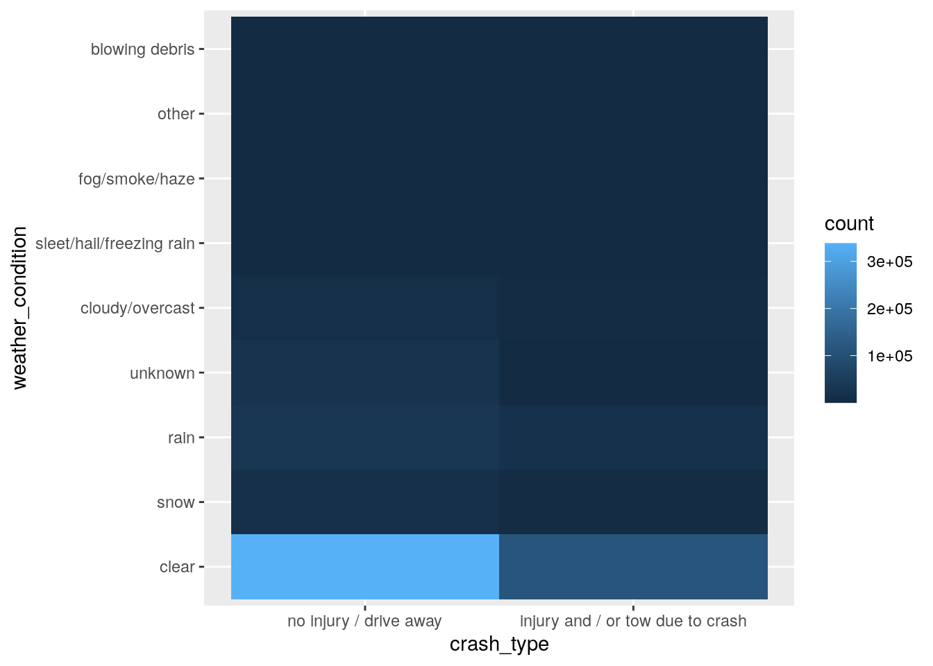
Although there are some differences, these appear to be pretty small. So, perhaps weather isn’t important for this model either.
Data preparation
Next, we’ll do a bit of preprocessing before training the models. This is where we’ll handle feature selection, data splitting, feature engineering, feature scaling, and creating the validation set (i.e., resampling).
The first thing we’ll do here is drop the variables that did not seem to have much of a relationship with crash_type during data exploration.
crashes <- select(crashes, -c(posted_speed_limit, weather_condition, alignment))
Next, let’s split the single data set into two: a training set and a testing set. A training data set is a data set of examples used during the learning process and is used to fit the models. A test data set is a data set that is independent of the training data set and is used to evaluate the performance of the final model. If a model fit to the training data set also fits the test data set well, we can be confident minimal overfitting has taken place. On the other hand, if the model seems to fit the training set better than the test set, we might have a case of overfitting.
For a data splitting strategy, let’s set aside 25% of the data for the test set. Since the outcome variable (crash_type) is somewhat imbalanced, we’ll also use a stratified random sample.
crash_split <- initial_split(crashes, strata = crash_type)
crash_train <- training(crash_split)
crash_test <- testing(crash_split)
Next, let’s create a base recipe for all models. Note the sequence of steps does matter here:
receipe():- Any variable on the left-hand side of the tilde (
~) is considered the model outcome (here,crash_type). The predictors of the model outcome appear on the right-hand side of the tilde. Here, we use the dot (.) to indicate all the other variables will be used as predictors. - A recipe is also associated with the data set used to create the model. This will usually be the training set, so
crash_trainhere.
- Any variable on the left-hand side of the tilde (
step_date(): Creates predictors for the year, month, and day of the week. Here, we’re selecting only the day of the week and month since there are limited observations for earlier years (e.g., 2013, 2014) in the data.step_rm(): Removes variables; here we use it to remove the original date variable since we no longer want it in the model.step_normalize(): Centers and scales numeric variables.step_dummy(): Converts characters or factors (i.e., nominal variables) into one or more numeric binary model terms for the levels of the original data.step_zv(): Removes indicator variables that only contain a single unique value (e.g. all zeros).
crash_recipe <- recipe(crash_type ~ ., data = crash_train) %>%
  step_date(date, features = c("dow", "month")) %>%
  step_rm(date) %>%
  step_normalize(all_numeric_predictors(), -all_outcomes()) %>%
  step_dummy(all_nominal_predictors(), -all_outcomes()) %>%
  step_zv(all_predictors(), -all_outcomes())
Recall that we already partitioned our data set into a training set and test set. This lets us judge whether a given model will generalize well to new data. However, using only two partitions may be insufficient when doing many rounds of hyperparameter tuning. So, it’s usually a good idea to create a validation set as well. We’ll use k-fold cross validation to build a set of 5 validation folds with the function vfold_cv, and we’ll also use stratified sampling to maintain the outcome class proportions.
k-fold cross validation randomly allocates the 571184 observations in the training set to 5 groups of roughly equal size, called “folds”. For the first iteration of resampling, the first fold is held out for the purpose of measuring performance. The other 80% of the data are used to fit the model. This model, trained on the analysis set, is applied to the assessment set to generate predictions. Then, performance statistics are computed based on those predictions.
In this case, 5-fold cross validation iteratively moves through the folds and leaves a different 20% out each time for model assessment. At the end of this process, there are 5 sets of performance statistics that were created on 5 data sets that were not used in the modeling process. While 5 models were created, these are not used further; we do not keep the models themselves trained on these folds because their only purpose is calculating performance metrics. The final resampling estimates for the model are the averages of the performance statistics replicates.
crashes_vfold <- vfold_cv(crash_train, v = 5, strata = crash_type)
We will come back to the validation set after we specified the models.
Model 1: Logistic regression
All available models are listed at
https://www.tidymodels.org/find/parsnip/. Since the outcome variable (crash_type) is categorical, a logistic regression model is a good place to start. Let’s use a model that can perform feature selection during training. The
glmnet R package fits a generalized linear model via penalized maximum likelihood. This method of estimating the logistic regression slope parameters uses a penalty on the process so that less relevant predictors are driven towards a value of zero. One of the glmnet penalization methods, called the
lasso method, can set the predictor slopes to zero if a large enough penalty is used.
To specify a penalized logistic regression model that uses a feature selection penalty, let’s use the parsnip package with the glmnet engine.
lr_mod <- logistic_reg(penalty = tune(), mixture = 1) %>%
  set_engine("glmnet") %>%
  set_mode("classification")
We’ll set the penalty argument to tune() as a placeholder for now. This is a model hyperparameter that we will
tune to find the best value for making predictions with our data. Setting mixture to a value of 1 means the glmnet model will potentially remove irrelevant predictors and choose a simpler model (i.e., via least absolute shrinkage and selection operator).
Create the workflow
Now, let’s bundle the model and recipe into a single workflow() object to make management of the R objects easier.
lr_workflow <- workflow() %>%
  add_model(lr_mod) %>%
  add_recipe(crash_recipe)
Train and tune the model
Before we fit this model, we need to set up a grid of penalty values to tune. Since there is only one hyperparameter to tune here, we can set the grid up manually using a one-column tibble with 30 candidate values.
lr_reg_grid <- tibble(penalty = 10^seq(-4, -1, length.out = 30))
Now we can use the validation set (crashes_vfold) to estimate the performance of our models by fitting the models on each of the folds and storing the results.
Let’s use tune_grid() to train these penalized logistic regression models. This will fit our model to each resample and evaluate on the heldout set from each resample. We’ll also save the validation set predictions (using control_grid()) so that diagnostic information can be available after the model fit. The area under the ROC curve, precision, recall, and F1-Score metrics will be used to quantify how well the model performs across a continuum of event thresholds.
lr_res <- lr_workflow %>%
  tune_grid(
    crashes_vfold,
    grid = lr_reg_grid,
    control = control_grid(save_pred = TRUE),
    metrics = metric_set(roc_auc, precision, recall, f_meas)
  )
Evaluate the model
Let’s take a look at the performance for every single fold.
lr_res %>%
  collect_metrics()
# A tibble: 120 × 7
    penalty .metric   .estimator  mean     n  std_err .config
      <dbl> <chr>     <chr>      <dbl> <int>    <dbl> <chr>
 1 0.0001   f_meas    binary     0.873     5 0.000454 Preprocessor1_Model01
 2 0.0001   precision binary     0.810     5 0.000335 Preprocessor1_Model01
 3 0.0001   recall    binary     0.947     5 0.000940 Preprocessor1_Model01
 4 0.0001   roc_auc   binary     0.784     5 0.000715 Preprocessor1_Model01
 5 0.000127 f_meas    binary     0.873     5 0.000454 Preprocessor1_Model02
 6 0.000127 precision binary     0.810     5 0.000335 Preprocessor1_Model02
 7 0.000127 recall    binary     0.947     5 0.000940 Preprocessor1_Model02
 8 0.000127 roc_auc   binary     0.784     5 0.000715 Preprocessor1_Model02
 9 0.000161 f_meas    binary     0.873     5 0.000454 Preprocessor1_Model03
10 0.000161 precision binary     0.810     5 0.000335 Preprocessor1_Model03
# … with 110 more rows
This isn’t very helpful on it’s own. Let’s visualize the validation set metrics by plotting the area under the ROC curve against the range of penalty values.
lr_res %>%
  collect_metrics() %>%
  filter(`.metric` == "roc_auc") %>%
  ggplot(aes(x = penalty, y = mean)) +
  geom_point() +
  geom_line() +
  ylab("Area under the ROC Curve") +
  scale_x_log10(labels = scales::label_number())
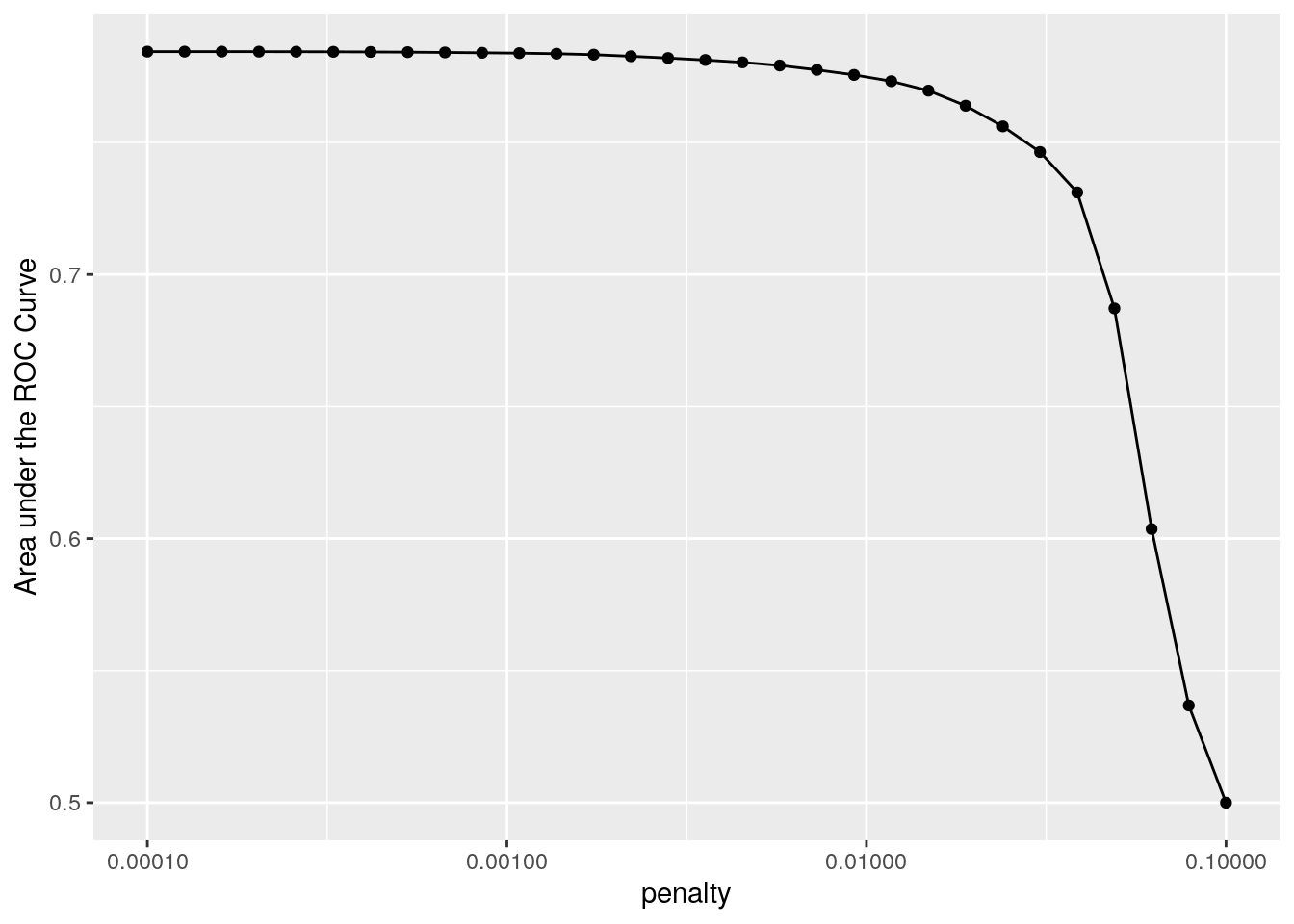
This plot suggests model performance is generally better at the smaller penalty values, meaning the majority of the predictors are important to the model. There’s also a steep drop in the area under the ROC curve towards the highest penalty values. This happens because a large enough penalty will remove all predictors from the model. And when there are no predictors in the model, predictive accuracy takes a nose dive.
Our model performance seems to plateau at the smaller penalty values, so judging performance by the roc_auc metric alone could lead to multiple options for the “best” value for this hyperparameter.
lr_res %>%
  show_best("roc_auc", n = 15) %>%
  arrange(penalty)
# A tibble: 15 × 7
    penalty .metric .estimator  mean     n  std_err .config
      <dbl> <chr>   <chr>      <dbl> <int>    <dbl> <chr>
 1 0.0001   roc_auc binary     0.784     5 0.000715 Preprocessor1_Model01
 2 0.000127 roc_auc binary     0.784     5 0.000715 Preprocessor1_Model02
 3 0.000161 roc_auc binary     0.784     5 0.000715 Preprocessor1_Model03
 4 0.000204 roc_auc binary     0.784     5 0.000717 Preprocessor1_Model04
 5 0.000259 roc_auc binary     0.784     5 0.000719 Preprocessor1_Model05
 6 0.000329 roc_auc binary     0.784     5 0.000724 Preprocessor1_Model06
 7 0.000418 roc_auc binary     0.784     5 0.000727 Preprocessor1_Model07
 8 0.000530 roc_auc binary     0.784     5 0.000732 Preprocessor1_Model08
 9 0.000672 roc_auc binary     0.784     5 0.000732 Preprocessor1_Model09
10 0.000853 roc_auc binary     0.784     5 0.000728 Preprocessor1_Model10
11 0.00108  roc_auc binary     0.784     5 0.000715 Preprocessor1_Model11
12 0.00137  roc_auc binary     0.784     5 0.000694 Preprocessor1_Model12
13 0.00174  roc_auc binary     0.783     5 0.000670 Preprocessor1_Model13
14 0.00221  roc_auc binary     0.783     5 0.000638 Preprocessor1_Model14
15 0.00281  roc_auc binary     0.782     5 0.000621 Preprocessor1_Model15
However, we may want to choose a penalty value further along the x-axis, closer to where we start to see the decline in model performance. For example, candidate model 12 with a penalty value of 0.00137 has basically the same performance as the numerically best model (model 1). However, model 12 might eliminate more predictors than model 1, and generally speaking, fewer irrelevant predictors is better. So if model performance is about the same, we should choose a model with a higher penalty value.
But keep in mind, we also collected other performance metrics. So, let’s take a look at those:
perf_metrics <- c("roc_auc", "precision", "recall", "f_meas")

get_metrics <- function(x) {
  lr_res %>%
    show_best(x, n = 15) %>%
    arrange(penalty)
}

map(perf_metrics, get_metrics)
[[1]]
# A tibble: 15 × 7
    penalty .metric .estimator  mean     n  std_err .config
      <dbl> <chr>   <chr>      <dbl> <int>    <dbl> <chr>
 1 0.0001   roc_auc binary     0.784     5 0.000715 Preprocessor1_Model01
 2 0.000127 roc_auc binary     0.784     5 0.000715 Preprocessor1_Model02
 3 0.000161 roc_auc binary     0.784     5 0.000715 Preprocessor1_Model03
 4 0.000204 roc_auc binary     0.784     5 0.000717 Preprocessor1_Model04
 5 0.000259 roc_auc binary     0.784     5 0.000719 Preprocessor1_Model05
 6 0.000329 roc_auc binary     0.784     5 0.000724 Preprocessor1_Model06
 7 0.000418 roc_auc binary     0.784     5 0.000727 Preprocessor1_Model07
 8 0.000530 roc_auc binary     0.784     5 0.000732 Preprocessor1_Model08
 9 0.000672 roc_auc binary     0.784     5 0.000732 Preprocessor1_Model09
10 0.000853 roc_auc binary     0.784     5 0.000728 Preprocessor1_Model10
11 0.00108  roc_auc binary     0.784     5 0.000715 Preprocessor1_Model11
12 0.00137  roc_auc binary     0.784     5 0.000694 Preprocessor1_Model12
13 0.00174  roc_auc binary     0.783     5 0.000670 Preprocessor1_Model13
14 0.00221  roc_auc binary     0.783     5 0.000638 Preprocessor1_Model14
15 0.00281  roc_auc binary     0.782     5 0.000621 Preprocessor1_Model15

[[2]]
# A tibble: 15 × 7
    penalty .metric   .estimator  mean     n   std_err .config
      <dbl> <chr>     <chr>      <dbl> <int>     <dbl> <chr>
 1 0.0001   precision binary     0.810     5 0.000335  Preprocessor1_Model01
 2 0.000127 precision binary     0.810     5 0.000335  Preprocessor1_Model02
 3 0.000161 precision binary     0.810     5 0.000335  Preprocessor1_Model03
 4 0.000204 precision binary     0.810     5 0.000318  Preprocessor1_Model04
 5 0.000259 precision binary     0.810     5 0.000304  Preprocessor1_Model05
 6 0.000329 precision binary     0.809     5 0.000309  Preprocessor1_Model06
 7 0.000418 precision binary     0.809     5 0.000309  Preprocessor1_Model07
 8 0.000530 precision binary     0.809     5 0.000329  Preprocessor1_Model08
 9 0.000672 precision binary     0.809     5 0.000339  Preprocessor1_Model09
10 0.000853 precision binary     0.808     5 0.000278  Preprocessor1_Model10
11 0.00108  precision binary     0.808     5 0.000251  Preprocessor1_Model11
12 0.00137  precision binary     0.807     5 0.000234  Preprocessor1_Model12
13 0.00174  precision binary     0.807     5 0.000218  Preprocessor1_Model13
14 0.00221  precision binary     0.806     5 0.000180  Preprocessor1_Model14
15 0.00281  precision binary     0.805     5 0.0000979 Preprocessor1_Model15

[[3]]
# A tibble: 15 × 7
   penalty .metric .estimator  mean     n  std_err .config
     <dbl> <chr>   <chr>      <dbl> <int>    <dbl> <chr>
 1 0.00356 recall  binary     0.956     5 0.000631 Preprocessor1_Model16
 2 0.00452 recall  binary     0.957     5 0.000670 Preprocessor1_Model17
 3 0.00574 recall  binary     0.960     5 0.000627 Preprocessor1_Model18
 4 0.00728 recall  binary     0.962     5 0.000723 Preprocessor1_Model19
 5 0.00924 recall  binary     0.967     5 0.000365 Preprocessor1_Model20
 6 0.0117  recall  binary     0.974     5 0.000515 Preprocessor1_Model21
 7 0.0149  recall  binary     0.981     5 0.000532 Preprocessor1_Model22
 8 0.0189  recall  binary     0.984     5 0.000379 Preprocessor1_Model23
 9 0.0240  recall  binary     0.990     5 0.000264 Preprocessor1_Model24
10 0.0304  recall  binary     0.993     5 0.000201 Preprocessor1_Model25
11 0.0386  recall  binary     0.996     5 0.000131 Preprocessor1_Model26
12 0.0489  recall  binary     0.996     5 0.000162 Preprocessor1_Model27
13 0.0621  recall  binary     1         5 0        Preprocessor1_Model28
14 0.0788  recall  binary     1         5 0        Preprocessor1_Model29
15 0.1     recall  binary     1         5 0        Preprocessor1_Model30

[[4]]
# A tibble: 15 × 7
    penalty .metric .estimator  mean     n  std_err .config
      <dbl> <chr>   <chr>      <dbl> <int>    <dbl> <chr>
 1 0.0001   f_meas  binary     0.873     5 0.000454 Preprocessor1_Model01
 2 0.000127 f_meas  binary     0.873     5 0.000454 Preprocessor1_Model02
 3 0.000161 f_meas  binary     0.873     5 0.000454 Preprocessor1_Model03
 4 0.000204 f_meas  binary     0.873     5 0.000448 Preprocessor1_Model04
 5 0.000259 f_meas  binary     0.873     5 0.000421 Preprocessor1_Model05
 6 0.000329 f_meas  binary     0.873     5 0.000422 Preprocessor1_Model06
 7 0.000530 f_meas  binary     0.873     5 0.000437 Preprocessor1_Model08
 8 0.000672 f_meas  binary     0.873     5 0.000428 Preprocessor1_Model09
 9 0.000853 f_meas  binary     0.873     5 0.000400 Preprocessor1_Model10
10 0.00108  f_meas  binary     0.873     5 0.000371 Preprocessor1_Model11
11 0.00137  f_meas  binary     0.873     5 0.000354 Preprocessor1_Model12
12 0.00174  f_meas  binary     0.873     5 0.000377 Preprocessor1_Model13
13 0.00221  f_meas  binary     0.873     5 0.000326 Preprocessor1_Model14
14 0.00281  f_meas  binary     0.873     5 0.000299 Preprocessor1_Model15
15 0.00356  f_meas  binary     0.873     5 0.000266 Preprocessor1_Model16
Let’s select model 15 in this case:
lr_best <- lr_res %>%
  select_best(metric = "f_meas")
Now we can use the predictions to create a confusion matrix with conf_mat().
lr_res %>%
  collect_predictions(parameters = lr_best) %>%
  conf_mat(crash_type, .pred_class)
                                  Truth
Prediction                         no injury / drive away
  no injury / drive away                           303912
  injury and / or tow due to crash                  14507
                                  Truth
Prediction                         injury and / or tow due to crash
  no injury / drive away                                      73671
  injury and / or tow due to crash                            36297
The confusion matrix can also be visualized in different formats using autoplot(). I personally like the heatmap type, but there are others that can be used as well.
lr_res %>%
  collect_predictions(parameters = lr_best)  %>%
  conf_mat(crash_type, .pred_class) %>%
  autoplot(type = "heatmap")

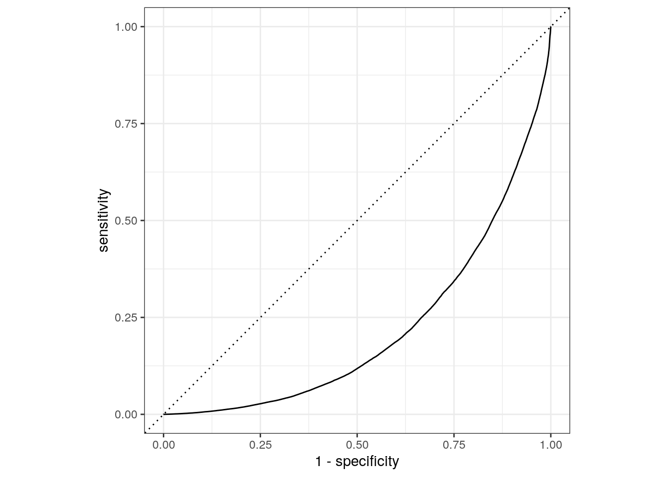
Let’s visualize the validation set ROC curve:
lr_auc <- lr_res %>%
  collect_predictions(parameters = lr_best) %>%
  roc_curve(crash_type, `.pred_injury and / or tow due to crash`) %>%
  mutate(model = "Logistic Regression")

autoplot(lr_auc)
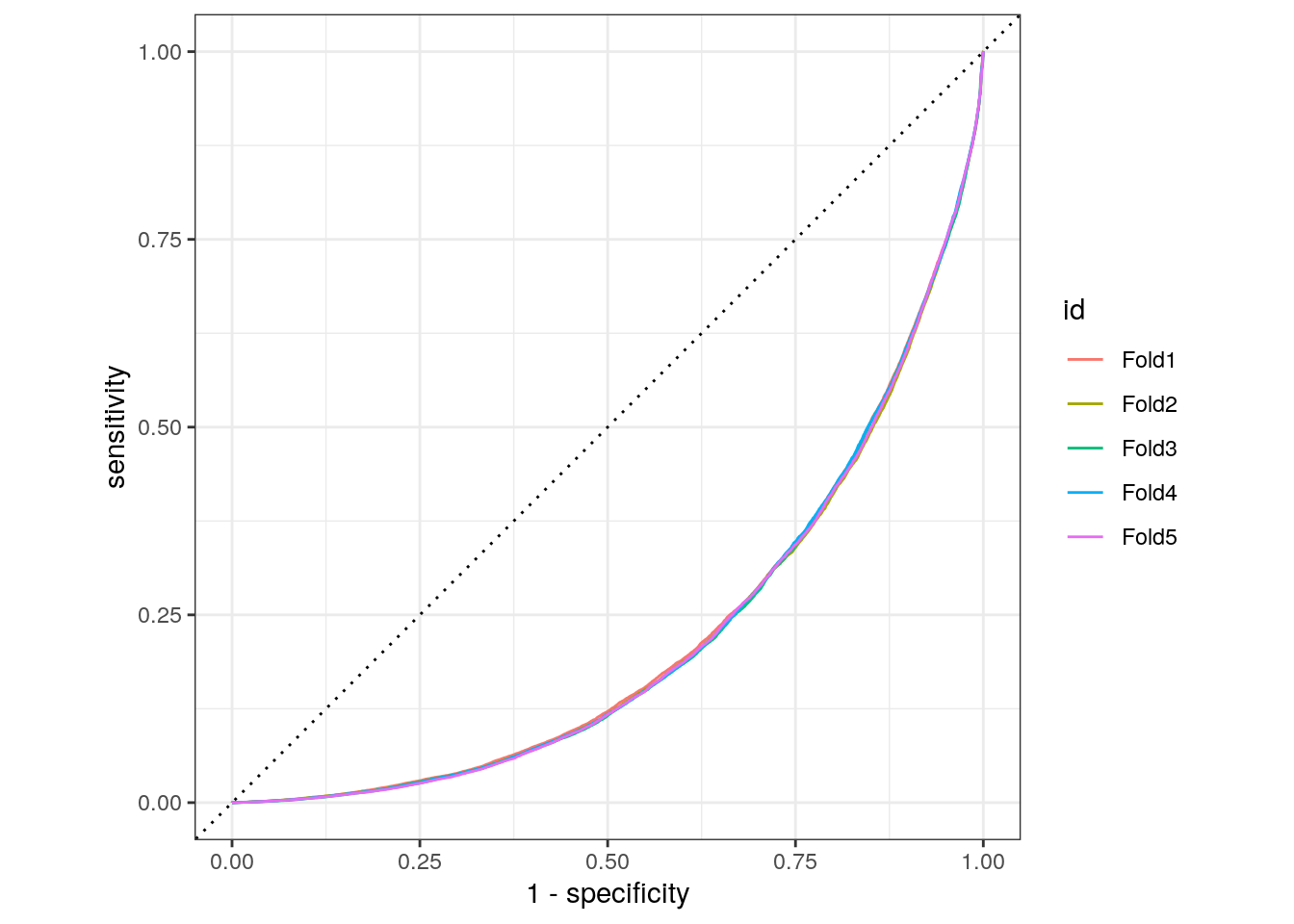
We can also make a ROC cure for the 5 folds. Since the category we are predicting is the injury/tow level in the crash_type factor, we provide roc_curve() with the relevant class probability .pred_injury and / or tow due to crash:
lr_res %>%
  collect_predictions(parameters = lr_best) %>%
  group_by(id) %>%
  roc_curve(crash_type, `.pred_injury and / or tow due to crash`) %>%
  autoplot()
Finally, we can also look at the predicted probability distributions for our two classes:
lr_res %>%
  collect_predictions(parameters = lr_best) %>%
  ggplot() +
  geom_density(
    aes(x = `.pred_injury and / or tow due to crash`,
        fill = crash_type),
    alpha = 0.5
  )
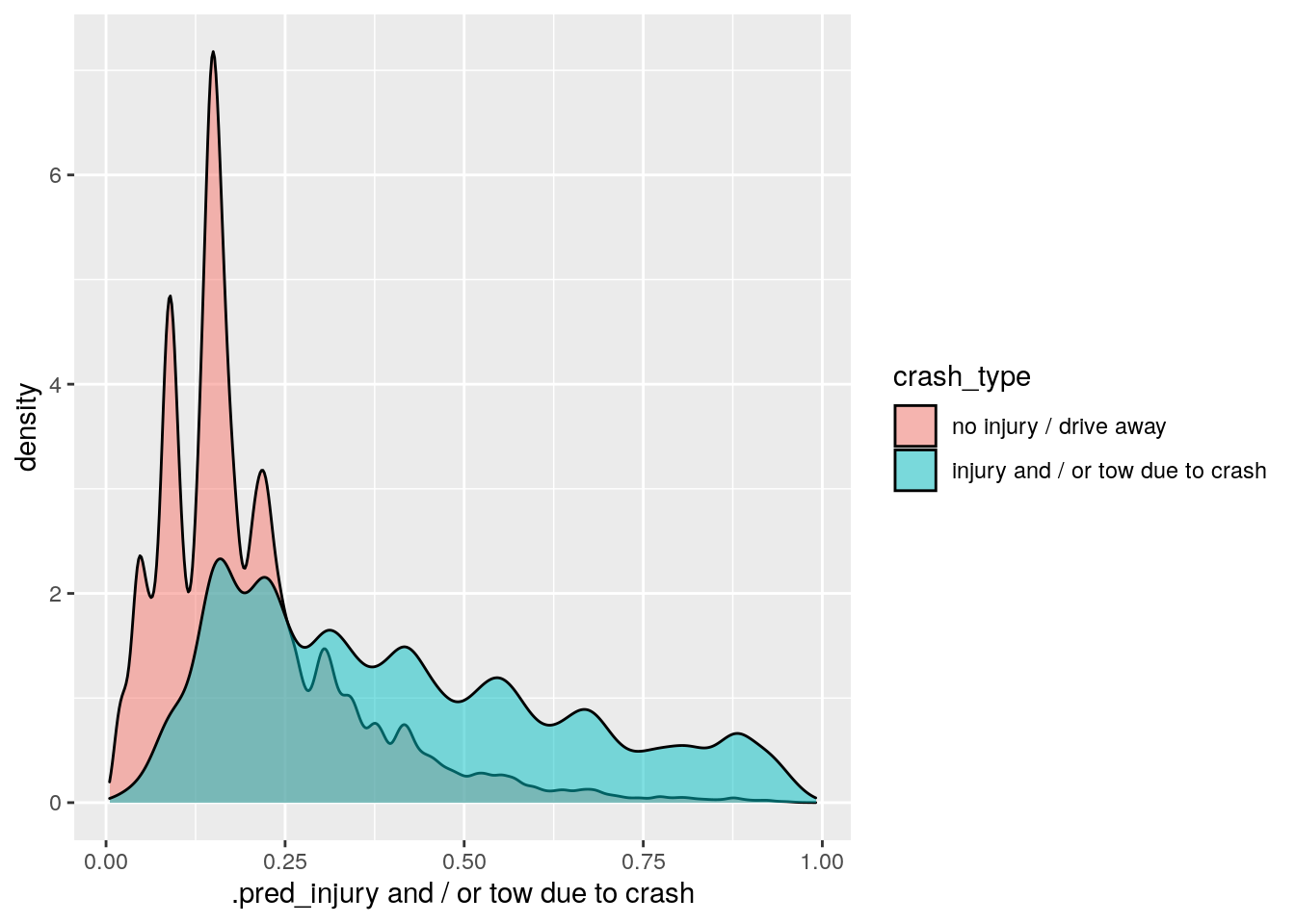
The level of performance generated by this logistic regression model isn’t great, but it’s better than an educated guess. Based on the frequency of crashes that result in injuries or vehicles being towed in the entire data set, we would expect about 24.6% of crashes to have these outcomes. However, based on the features we’ve selected here, our model correctly predicted these crash types about 33% of the time. So, we’ve improved our predictions, but only by about 8%. Perhaps the linear nature of the prediction equation could be limiting our model’s performance. As a next step, we might consider using a non-linear model, like a tree-based ensemble method.
Model 2: Random forest
An effective, low-maintenance, non-linear modeling approach is a random forest, which tends to be more flexible than logistic regression. A random forest is an ensemble model that often consists of thousands of decision trees. Each individual tree sees a slightly different version of the training set and learns a sequence of splitting rules to predict new data. Random forests require very little preprocessing and can handle many types of predictors (e.g., skewed, continuous, categorical, etc.). Although the default hyperparameters for random forests tend to give reasonable results, we’ll tune two hyperparameters that could improve performance. This should also help since we’ll be limiting the number of trees used to 20 to speed up the time it takes to fit the model.
rf_mod <- rand_forest(mtry = tune(), min_n = tune(), trees = 20) %>%
  set_engine("ranger", importance = "impurity") %>%
  set_mode("classification")
For the hyperparameters in this model, we use tune() as a placeholder for the mtry and min_n argument values. The mtry hyperparameter sets the number of predictor variables that each node in the decision tree sees and learns about. The min_n hyperparameter sets the minimum n to split at any node. We also added importance = "impurity" when setting the engine. This will provide variable importance scores for this model, which gives some insight into which predictors drive model performance.
Create the workflow
Next, let’s bundle the recipe and model.
rf_workflow <- workflow() %>%
  add_model(rf_mod) %>%
  add_recipe(crash_recipe)
Train and tune the model
Since we have more than one hyperparameter to tune in this model, let’s use a space-filling design with 25 candidate models.
rf_res <- rf_workflow %>%
  tune_grid(
    crashes_vfold,
    grid = 25,
    control = control_grid(save_pred = TRUE),
    metrics = metric_set(roc_auc, precision, recall, f_meas)
  )
i Creating pre-processing data to finalize unknown parameter: mtry
Evaluate the model
Out of the 25 candidates, here are the top 5 random forest models based on their F1-Scores:
rf_res %>%
  show_best(metric = "f_meas")
# A tibble: 5 × 8
   mtry min_n .metric .estimator  mean     n  std_err .config
  <int> <int> <chr>   <chr>      <dbl> <int>    <dbl> <chr>
1     6    19 f_meas  binary     0.874     5 0.000433 Preprocessor1_Model20
2     5    27 f_meas  binary     0.874     5 0.000388 Preprocessor1_Model03
3    16    31 f_meas  binary     0.872     5 0.000379 Preprocessor1_Model24
4    22    39 f_meas  binary     0.872     5 0.000454 Preprocessor1_Model10
5    13     7 f_meas  binary     0.871     5 0.000403 Preprocessor1_Model16
Let’s select the best model according to the F1-Score. Our final tuning parameter values are:
rf_best <- rf_res %>%
  select_best(metric = "f_meas")

rf_best
# A tibble: 1 × 3
   mtry min_n .config
  <int> <int> <chr>
1     6    19 Preprocessor1_Model20
To calculate the data needed to plot the ROC curve, we use collect_predictions(). This is only possible after tuning with control_grid(save_pred = TRUE). Now, we can use the predictions to create a confusion matrix with conf_mat().
rf_res %>%
  collect_predictions() %>%
  conf_mat(crash_type, .pred_class)
                                  Truth
Prediction                         no injury / drive away
  no injury / drive away                          7349427
  injury and / or tow due to crash                 611048
                                  Truth
Prediction                         injury and / or tow due to crash
  no injury / drive away                                    1662563
  injury and / or tow due to crash                          1086637
To filter the predictions for only our best random forest model, we can use the parameters argument and pass it our tibble with the best hyperparameter values from tuning, which we called rf_best.
rf_auc <- rf_res %>%
  collect_predictions(parameters = rf_best) %>%
  roc_curve(crash_type, `.pred_injury and / or tow due to crash`) %>%
  mutate(model = "Random Forest")

autoplot(rf_auc)

Compare models
Now, it’s time to compare the models. The first thing we’ll do is extract the performance metrics from each of the models and combine them into a single data frame.
lr_metrics <- lr_res %>%
  collect_metrics() %>%
  mutate(model = "Logistic Regression")

rf_metrics <- rf_res %>%
  collect_metrics() %>%
  mutate(model = "Random Forest")

compare_mod <- bind_rows(lr_metrics, rf_metrics)
Fist, let’s take a look at the average F1-Score for each model:
compare_mod %>%
  filter(.metric == "f_meas") %>%
  group_by(model) %>%
  summarize(avg_f_meas = mean(mean)) %>%
  mutate(model = fct_reorder(model, avg_f_meas)) %>%
  ggplot(aes(model, avg_f_meas, fill = model)) +
  geom_col() +
  coord_flip() +
  scale_fill_brewer(palette = "Blues") +
  geom_text(
    size = 5,
    aes(label = round_half_up(avg_f_meas, 2), y = avg_f_meas - .8)
  )
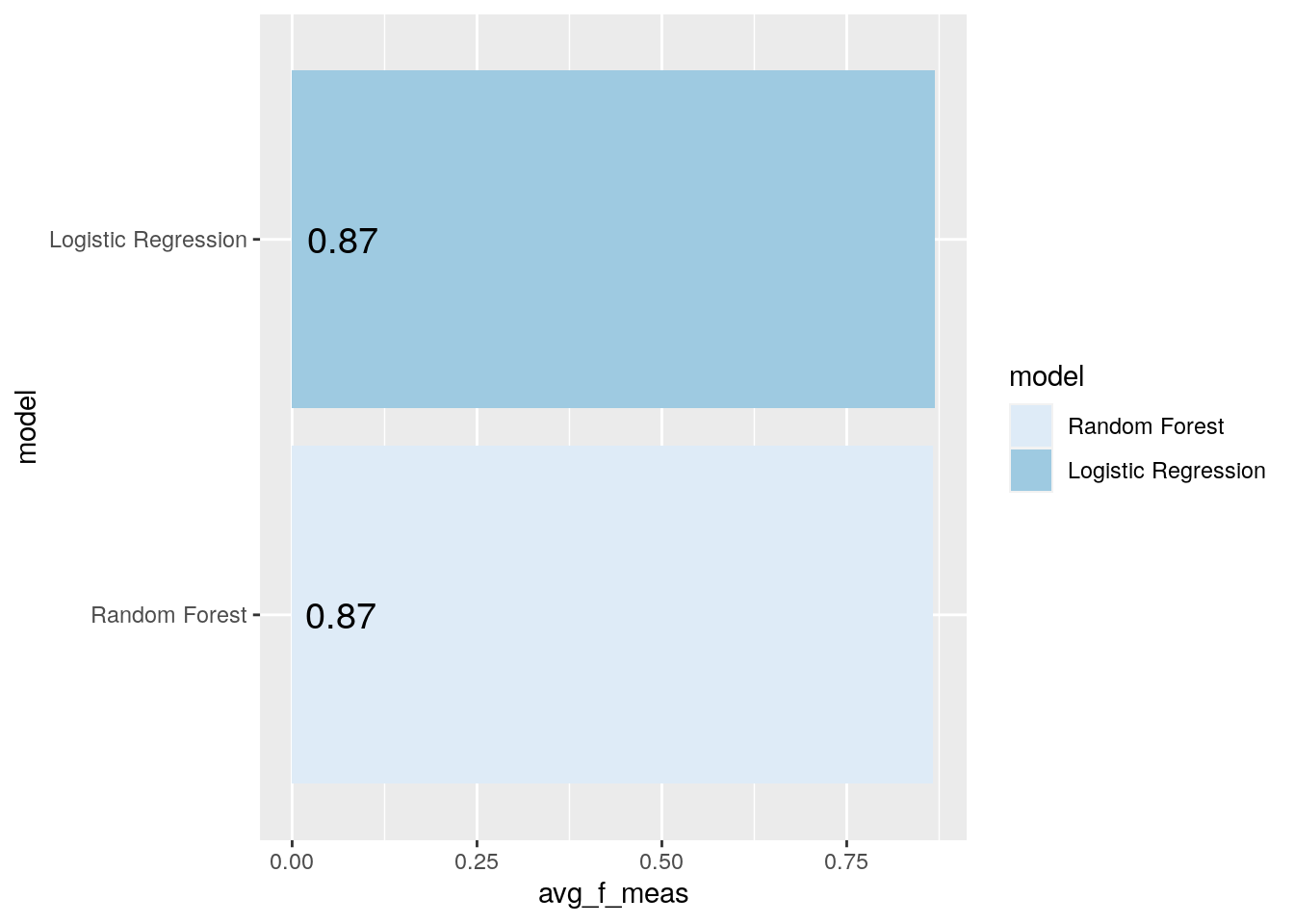
Not much of a difference here. So, we may also want to check out the average ROC curve for each model:
compare_mod %>%
  filter(.metric == "roc_auc") %>%
  group_by(model) %>%
  summarize(avg_roc = mean(mean)) %>%
  mutate(model = fct_reorder(model, avg_roc)) %>%
  ggplot(aes(model, avg_roc, fill = model)) +
  geom_col() +
  coord_flip() +
  scale_fill_brewer(palette = "Blues") +
  geom_text(
    size = 5,
    aes(label = round_half_up(avg_roc, 2), y = avg_roc - .7)
  )
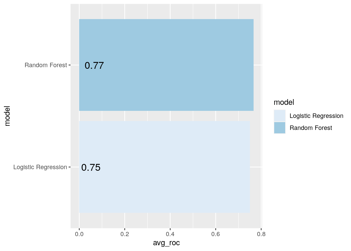
Looks like our random forest model did a bit better here, but still pretty close. Let’s plot the validation set ROC curves for the top penalized logistic regression model and random forest model:
bind_rows(rf_auc, lr_auc) %>%
  ggplot(aes(x = 1 - specificity, y = sensitivity, col = model)) +
  geom_path(lwd = 1.5, alpha = 0.8) +
  geom_abline(lty = 3) +
  coord_equal() +
  scale_color_viridis_d(option = "plasma", end = .6)
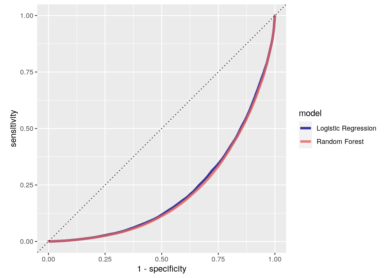
Overall, the model results are pretty similar, but the random forest model did seem to perform better than the logistic regression model. In this case, I highlighted the ROC AUC and F1-Score performance metrics, but the “best” performance metric will always depend on the question you are trying to answer with your model. For example, in some cases, you might be much more concerned about false negatives than you are false positives (e.g., when predicting severe storms). In other situations, you might only be concerned about each these to the extent they influence a model’s precision (e.g., when predicting profitable stocks).
To keep things simple, let’s stick with the ROC AUC metric in this case. AUC stands for area under the curve. What curve, you may ask? The ROC curve, specifically. The ROC curve plots the tradeoff between the true positive rate (sensitivity) and and false positive rate (1 - specificity). Ideally, we want to maximize the true positive rate and minimize the false positive rate.
Let’s find the maximum mean ROC AUC:
compare_mod %>%
filter(.metric == "roc_auc") %>%
group_by(model) %>%
summarize(avg_roc_auc = mean(mean)) %>%
slice_max(avg_roc_auc)
[38;5;246m# A tibble: 1 × 2[39m
model avg_roc_auc
[3m[38;5;246m<chr>[39m[23m [3m[38;5;246m<dbl>[39m[23m
[38;5;250m1[39m Random Forest 0.766
Now, it’s time to fit the best model one last time to the full training set. Then, we can evaluate the resulting final model on the test set.
Last fit
Recall that our goal was to predict whether a traffic crash would result in an injury or a vehicle being towed based on a priori situational factors. Given the results, we determined the random forest model performed better than the penalized logistic regression model. We also know learned the best model hyperparameters from the rf_best object we created earlier. Now, we just need to fit the final model on all the rows of data not originally held out for testing (i.e., the training and validation sets) and evaluate the model performance one more time with the test set.
The
tune package contains the function last_fit(), which fits a model to the whole training data and evaluates it on the test set. We just need to provide the workflow object of the best model and data split object (not the training data).
last_rf_mod <- rand_forest(
    mtry = rf_best$mtry,
    min_n = rf_best$min_n,
    trees = 20
  ) %>%
  set_engine("ranger", importance = "impurity") %>%
  set_mode("classification")

last_rf_workflow <- rf_workflow %>%
  update_model(last_rf_mod)

last_rf_fit <- last_rf_workflow %>%
  last_fit(crash_split)
And these are the final performance metrics:
last_rf_fit %>%
collect_metrics()
[38;5;246m# A tibble: 2 × 4[39m
.metric .estimator .estimate .config
[3m[38;5;246m<chr>[39m[23m [3m[38;5;246m<chr>[39m[23m [3m[38;5;246m<dbl>[39m[23m [3m[38;5;246m<chr>[39m[23m
[38;5;250m1[39m accuracy binary 0.795 Preprocessor1_Model1
[38;5;250m2[39m roc_auc binary 0.787 Preprocessor1_Model1
Remember, if a model fit to the training data set also fits the test data set well, we can be reasonably confident that minimal overfitting has taken place.
To learn more about the model, we can look at the variable importance scores in the .workflow column. We pluck the first element from the column, and pull out the fit from the workflow object. Then, we can use the
vip package to visualize the variable importance scores for the top features.
last_rf_fit %>%
  pluck(".workflow", 1) %>%
  extract_fit_parsnip() %>%
  vip(num_features = 10)
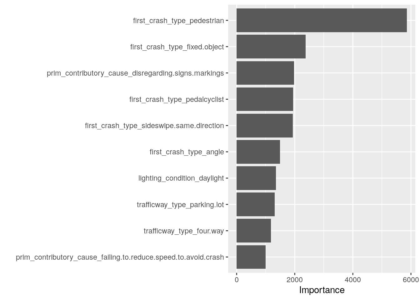
By far, the most important factor in whether a crash results in injuries or the vehicle being towed is if the first collision in the crash involved a pedestrian or not.
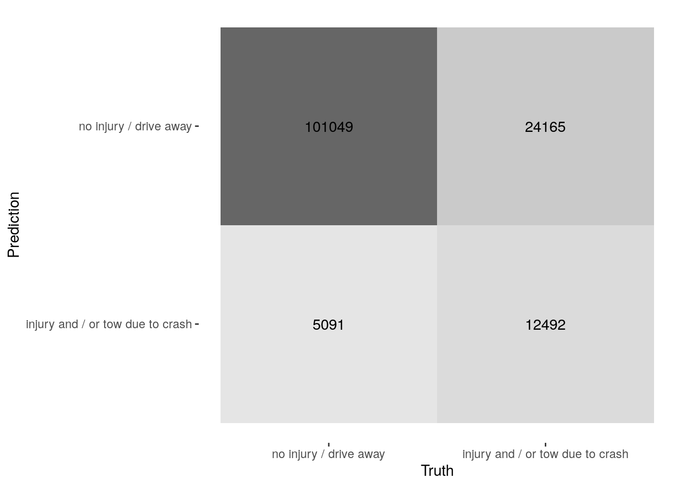
Let’s take a quick look at the confusion matrix:
last_rf_fit %>%
  collect_predictions() %>%
  conf_mat(crash_type, .pred_class) %>%
  autoplot(type = "heatmap")
And, let’s create the final ROC curve:
last_rf_fit %>%
  collect_predictions() %>%
  roc_curve(crash_type, `.pred_injury and / or tow due to crash`) %>%
  autoplot()
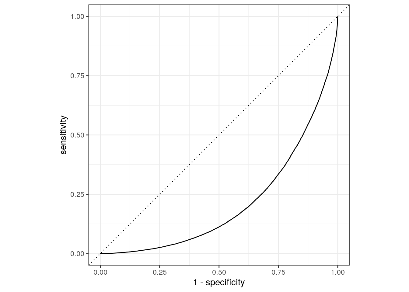
The results from the validation set and test set performance statistics are very close, so we can be reasonably confident the random forest model with the selected features and hyperparameters would perform well when predicting new data.
Special thanks to Drew Triplett for his helpful comments on an earlier draft of this post!